Machine Learning Rocks Week 1 on coursera.
After a failed attempt to do the machine learning course on Coursera earlier this year, I was inspired to take another stab at it when I saw that it was being run again. The last time, I was intimidated by the heavy use of math and the thetas and alphas really scared me. But now, in another brave attempt, I enrolled into the course again and found the math to be beautiful.
Week 1 of the course might just be a basic introduction to the techniques and scope of machine learning, but it blew my mind, in the sense that I could actually visualise the first algorithm that the lectures taught me. Here’s a summary of what I learnt.
Machine Learning is the process of teaching a machine to do a job. In the broad scope of things, an automation script you wrote, could be considered machine learning, but specifically, your algorithm must be able to predict things, be able to find meaning in a large amount of data based on some criteria. So how do we go about doing this?
The course first teaches you about the two different types of ML -
-
Supervised Learning - If you have to train your machine to do a certain job by teaching how it was performed previously ie with existing cause and result data, then that is supervised learning. This kind is pretty straightforward and the upcoming example of predicting house prices based on criteria like size and age of the house is a common world application. Weather prediction, stock price prediction etc come under this umbrella.
-
Unsupervised Learning - If you just provide your machine with a large volume of data and expect classification results from it, then it is unsupervised learning. I’m a bit hazy in the understanding of this branch of ML. The examples the professor cited were of clustering data with applications like market segment discovery, grouping of newspaper articles. I’m not very sure of how this works. Maybe it will become clearer as the course progresses.
I liked the way ML was defined
“A computer program is said to learn from experience E with respect to some task T and some performance measure P, if its performance on T, as measured by P, improves with experience E”
thus explaining to the student clearly that any ML problem would comprise of a task T, measure P and an experience E. This was a very concise definition.
For the first week, the course focused on Linear regression with one variable and the corresponding Gradient Descent Algorithm for finding the optimum linear equation.
The problem posed was this - Task - Be able to predict the cost of a house based on its square footage. Experience - The training data is a set of previous home sales ie a set of corresponding prices and home sizes. Performance - Find the linear curve that has minimum error tolerance for all the data in the training set.
The training set looks something like this -
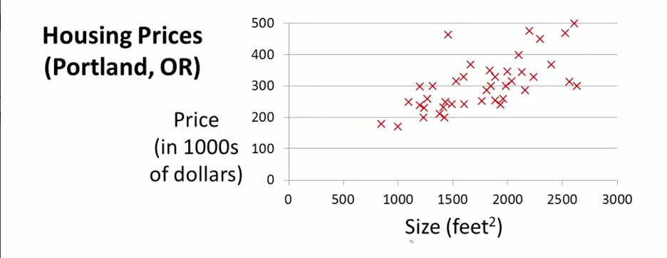
In simple words, the objective is to find a line passing through this data that includes all the data points.
The equation for a straight line is
hθ = θ0 + θ1x
Our ideal line is y = θ0 + θ1x
The solution to the problem would be to get a minimum (hθ - y)
To re iterate, our objective is to find θ0 and θ1 to suit the above criteria.
..to be continued..
blog comments powered by Disqus